Introduction to Data Frames#
Case Study: Diamonds#
In this lesson, we’re going to do some basic data analyses on a set of diamond characteristics and prices. First, we’ll download the data:
!gdown 1Q2saE5Wjis_4Hc3V5MBzAh3ei_bF2Q9M
If you open the file in a text editor, you will see that it consists of a bunch of lines, each with a bunch of commas. This is a csv or “comma-separated value” file. Every row represents a record (like a row in a spreadsheet), with each cell separated by a comma. The first row has the same format, but the entries are the names of the columns.
Loading the data#
We would like to load this data into Python. But to do so, we will need to tell Python that we want to get some tools ready. These tools are located in a library (the Python term is “module”) called Pandas. So we do this:
import pandas as pd
This tells Python to load the pandas module and nickname it pd. Then, whenever we want to use functionality from pandas, we do so by giving the address of the function we want. In this case, we want to load data from a csv file, so we call the function read_csv:
data = pd.read_csv('minerals.csv')
Let’s read from the left:
data =
tells Python that we want to do something (on the right hand side of the equation) and assign its output to a variable called data. We could have called it duck or shotput or harmony, but we want to give our variables meaningful names, and in cases where we are only going to be exploring a single dataset, it’s convenient to name it the obvious thing.
On the right hand side, we’re doing several things:
We’re telling Python to look in the
pandasmodule (nicknamedpd)We telling Python to call a function named
read_csvthat’s found there (we will find that looking up functions in modules is a lot like looking up files in directories)We’re giving the function the (local) path to the file in quotes
We will see this pattern repeatedly in Python. We use names like read_csv to tell Python to perform actions. As we saw before we supply variables or pieces of information (“arguments”) needed as inputs by Python to perform those actions.
Examining the data#
So what did we accomplish?
The easiest way to see is by asking Python to print the variable to the screen. We can do this with
print(data)
        item shape  carat cut color clarity polish symmetry  depth  table  \
0          1    PS   0.28   F     F     SI2     VG        G   61.6   50.0
1          2    PS   0.23   G     F     SI1     VG        G   67.5   51.0
2          3    EC   0.34   G     I     VS2     VG       VG   71.6   65.0
3          4    MQ   0.34   G     J     VS1      G        G   68.2   55.0
4          5    PS   0.23   G     D     SI1     VG       VG   55.0   58.0
...      ...   ...    ...  ..   ...     ...    ...      ...    ...    ...
65371  65372    RD  10.13   I     F      IF     EX       EX   60.3   58.0
65372  65373    RD  20.13   I     J     VS1     EX       EX   59.2   59.0
65373  65374    RD  12.35   I     G      IF     EX       EX   59.8   60.0
65374  65375    RD   9.19   I     E      IF     EX       EX   60.9   60.0
65375  65376    RD  10.13   I     D      FL     EX       EX   62.5   57.0

      fluorescence  price per carat       culet  length to width ratio  \
0            Faint              864         NaN                   1.65
1              NaN             1057         NaN                   1.46
2            Faint              812         NaN                   1.40
3            Faint              818         NaN                   1.52
4              NaN             1235         NaN                   1.42
...            ...              ...         ...                    ...
65371          NaN           130112  Very Small                   1.01
65372          NaN            66420         NaN                   1.01
65373        Faint           110662         NaN                   1.01
65374          NaN           150621         NaN                   1.00
65375          NaN           256150         NaN                   1.00

             delivery date      price
0       \nJul 8\n      242.0
1       \nJul 8\n      243.0
2      \nJul 12\n      276.0
3       \nJul 8\n      278.0
4      \nJul 14\n      284.0
...                    ...        ...
65371   \nJul 8\n  1318034.0
65372  \nJul 14\n  1337035.0
65373  \nJul 12\n  1366679.0
65374  \nJul 13\n  1384207.0
65375  \nJul 12\n  2594800.0

[65376 rows x 16 columns]
You should be able to see that the data consists of a bunch of rows and columns, and that, at some point in the middle, Python puts a bunch of …’s, indicating it’s not printing all the information. That’s good in this case, since the data are pretty big.
So how big are the data? We can find this out by typing
data.shape
(65376, 16)
Note
We could have gotten the same answer by typing
print(data.shape)
but, as we’ve seen several times now, when we just type the variable name, Python assumes we mean print.
So what does this answer mean? It means that our data set has something like 65,000 rows and 16 columns. Here, the convention is (rows, columns).
Notice also that the way we got this piece of information was by typing the variable, followed by ., followed by the name of some property of the data (called an “attribute”). Again, you can think of this variable as an object having both pieces of information (attributes) and pieces of behavior (functions or methods) tucked inside of it like a file system. The way we access those is by giving a path, except with . instead of /.
But there’s an even friendlier way to look at our data that’s special to the notebook. To look at the first few rows of our data, we can type
data.head()
| item | shape | carat | cut | color | clarity | polish | symmetry | depth | table | fluorescence | price per carat | culet | length to width ratio | delivery date | price | |
|---|---|---|---|---|---|---|---|---|---|---|---|---|---|---|---|---|
| 0 | 1 | PS | 0.28 | F | F | SI2 | VG | G | 61.6 | 50.0 | Faint | 864 | NaN | 1.65 | \nJul 8\n | 242.0 |
| 1 | 2 | PS | 0.23 | G | F | SI1 | VG | G | 67.5 | 51.0 | NaN | 1057 | NaN | 1.46 | \nJul 8\n | 243.0 |
| 2 | 3 | EC | 0.34 | G | I | VS2 | VG | VG | 71.6 | 65.0 | Faint | 812 | NaN | 1.40 | \nJul 12\n | 276.0 |
| 3 | 4 | MQ | 0.34 | G | J | VS1 | G | G | 68.2 | 55.0 | Faint | 818 | NaN | 1.52 | \nJul 8\n | 278.0 |
| 4 | 5 | PS | 0.23 | G | D | SI1 | VG | VG | 55.0 | 58.0 | NaN | 1235 | NaN | 1.42 | \nJul 14\n | 284.0 |
This gives 5 rows by default (note that counting starts at 0!), but we can easily ask Python for 10:
data.head(10)
| item | shape | carat | cut | color | clarity | polish | symmetry | depth | table | fluorescence | price per carat | culet | length to width ratio | delivery date | price | |
|---|---|---|---|---|---|---|---|---|---|---|---|---|---|---|---|---|
| 0 | 1 | PS | 0.28 | F | F | SI2 | VG | G | 61.6 | 50.0 | Faint | 864 | NaN | 1.65 | \nJul 8\n | 242.0 |
| 1 | 2 | PS | 0.23 | G | F | SI1 | VG | G | 67.5 | 51.0 | NaN | 1057 | NaN | 1.46 | \nJul 8\n | 243.0 |
| 2 | 3 | EC | 0.34 | G | I | VS2 | VG | VG | 71.6 | 65.0 | Faint | 812 | NaN | 1.40 | \nJul 12\n | 276.0 |
| 3 | 4 | MQ | 0.34 | G | J | VS1 | G | G | 68.2 | 55.0 | Faint | 818 | NaN | 1.52 | \nJul 8\n | 278.0 |
| 4 | 5 | PS | 0.23 | G | D | SI1 | VG | VG | 55.0 | 58.0 | NaN | 1235 | NaN | 1.42 | \nJul 14\n | 284.0 |
| 5 | 6 | MQ | 0.23 | F | G | VS2 | VG | G | 71.6 | 55.0 | NaN | 1248 | NaN | 1.95 | \nJul 8\n | 287.0 |
| 6 | 7 | RA | 0.37 | F | I | SI2 | G | G | 79.0 | 76.0 | NaN | 781 | NaN | 1.03 | \nJul 8\n | 289.0 |
| 7 | 8 | EC | 0.24 | VG | E | SI1 | VG | VG | 68.6 | 65.0 | Faint | 1204 | NaN | 1.34 | \nJul 8\n | 289.0 |
| 8 | 9 | RD | 0.24 | I | G | SI2 | VG | VG | 62.0 | 59.0 | NaN | 1204 | NaN | 1.01 | \nJul 8\n | 289.0 |
| 9 | 10 | MQ | 0.33 | G | H | SI2 | G | G | 66.7 | 61.0 | Medium | 888 | NaN | 2.02 | \nJul 8\n | 293.0 |
Here, head is a method of the variable data (meaning it’s a function stored in the data object). In the second case, we explicitly told head how many rows we wanted, while in the first, the number defaulted to 5.
Likewise, we can ask for the last few rows of the dataset with tail:
data.tail(7)
| item | shape | carat | cut | color | clarity | polish | symmetry | depth | table | fluorescence | price per carat | culet | length to width ratio | delivery date | price | |
|---|---|---|---|---|---|---|---|---|---|---|---|---|---|---|---|---|
| 65369 | 65370 | RD | 9.56 | I | F | FL | EX | EX | 60.3 | 60.0 | NaN | 120336 | Very Small | 1.01 | \nJul 8\n | 1150413.0 |
| 65370 | 65371 | CU | 8.40 | G | D | IF | VG | G | 57.9 | 59.0 | NaN | 144300 | Slightly Large | 1.20 | \nJul 8\n | 1212120.0 |
| 65371 | 65372 | RD | 10.13 | I | F | IF | EX | EX | 60.3 | 58.0 | NaN | 130112 | Very Small | 1.01 | \nJul 8\n | 1318034.0 |
| 65372 | 65373 | RD | 20.13 | I | J | VS1 | EX | EX | 59.2 | 59.0 | NaN | 66420 | NaN | 1.01 | \nJul 14\n | 1337035.0 |
| 65373 | 65374 | RD | 12.35 | I | G | IF | EX | EX | 59.8 | 60.0 | Faint | 110662 | NaN | 1.01 | \nJul 12\n | 1366679.0 |
| 65374 | 65375 | RD | 9.19 | I | E | IF | EX | EX | 60.9 | 60.0 | NaN | 150621 | NaN | 1.00 | \nJul 13\n | 1384207.0 |
| 65375 | 65376 | RD | 10.13 | I | D | FL | EX | EX | 62.5 | 57.0 | NaN | 256150 | NaN | 1.00 | \nJul 12\n | 2594800.0 |
If you look carefully, you might notice that the rows seem to be sorted by the last item, price. The odd characters under delivery data are a result of the process used to download these data from the internet.
Finally, as a first, pass, we might just want to know some simple summary statistics of our data:
data.describe()
| item | carat | depth | table | price per carat | length to width ratio | price | |
|---|---|---|---|---|---|---|---|
| count | 65376.000000 | 65376.000000 | 65376.000000 | 65376.000000 | 65376.000000 | 65376.000000 | 6.537600e+04 |
| mean | 32688.500000 | 0.878652 | 63.245745 | 59.397770 | 6282.785365 | 1.111838 | 9.495346e+03 |
| std | 18872.569936 | 0.783895 | 3.861799 | 4.868447 | 7198.173546 | 0.212317 | 3.394968e+04 |
| min | 1.000000 | 0.230000 | 6.700000 | 6.000000 | 781.000000 | 0.770000 | 2.420000e+02 |
| 25% | 16344.750000 | 0.400000 | 61.200000 | 57.000000 | 2967.000000 | 1.010000 | 1.121000e+03 |
| 50% | 32688.500000 | 0.700000 | 62.200000 | 58.000000 | 4150.000000 | 1.010000 | 2.899000e+03 |
| 75% | 49032.250000 | 1.020000 | 64.400000 | 61.000000 | 6769.000000 | 1.110000 | 6.752250e+03 |
| max | 65376.000000 | 20.130000 | 80.000000 | 555.000000 | 256150.000000 | 3.120000 | 2.594800e+06 |
The fine art of looking things up#
The Python ecosystem is huge. Nobody knows all the functions for all the libraries. This means that when you start analyzing data in earnest, you will need to learn the parts important for solving your particular problem. Initially, this will be difficult; everything will be new to you. Eventually, though, you develop a conceptual base that will be easy to add to.
So what should you do in this case? How do we learn more about the functions we’ve used so far?
First off, let’s figure out what type of object data is. Every variable in Python is an object (meaning it has both information and behavior stored inside of it), and every object has a type. We can find this by using the type function:
type(1)
int
Here, int means integer, a number with no decimal part.
type(1.5)
float
Float is anything with a decimal point. Be aware that the precision of float variables is limited, and there is the potential for roundoff errors in calculations if you ever start to do serious data crunching (though most of the time you’ll be fine).
type(data)
pandas.core.frame.DataFrame
So what in the world is this?
Read it like so: the type of object data is is defined in the pandas module, in the core submodule, in the frame sub-submodule, and it is DataFrame. Again, using our filesystem analogy, the data variable has type DataFrame, and Python gives us the full path to its definition. As we will see, dataframes are a very convenient type of object in which to store our data, since this type of object carries with it very powerful behaviors (methods) that can be used to clean and analyze data.
So if type tells us the type of object, how do we find out what’s in it?
We can do that with the dir command. dir is short for “directory,” and tells us the name of all the attributes (information) and methods (behaviors) associated with an object:
dir(data)
['T',
 '_AXIS_LEN',
 '_AXIS_ORDERS',
 '_AXIS_TO_AXIS_NUMBER',
 '_HANDLED_TYPES',
 '__abs__',
 '__add__',
 '__and__',
 '__annotations__',
 '__array__',
 '__array_priority__',
 '__array_ufunc__',
 '__arrow_c_stream__',
 '__bool__',
 '__class__',
 '__contains__',
 '__copy__',
 '__dataframe__',
 '__dataframe_consortium_standard__',
 '__deepcopy__',
 '__delattr__',
 '__delitem__',
 '__dict__',
 '__dir__',
 '__divmod__',
 '__doc__',
 '__eq__',
 '__finalize__',
 '__firstlineno__',
 '__floordiv__',
 '__format__',
 '__ge__',
 '__getattr__',
 '__getattribute__',
 '__getitem__',
 '__getstate__',
 '__gt__',
 '__hash__',
 '__iadd__',
 '__iand__',
 '__ifloordiv__',
 '__imod__',
 '__imul__',
 '__init__',
 '__init_subclass__',
 '__invert__',
 '__ior__',
 '__ipow__',
 '__isub__',
 '__iter__',
 '__itruediv__',
 '__ixor__',
 '__le__',
 '__len__',
 '__lt__',
 '__matmul__',
 '__mod__',
 '__module__',
 '__mul__',
 '__ne__',
 '__neg__',
 '__new__',
 '__nonzero__',
 '__or__',
 '__pandas_priority__',
 '__pos__',
 '__pow__',
 '__radd__',
 '__rand__',
 '__rdivmod__',
 '__reduce__',
 '__reduce_ex__',
 '__repr__',
 '__rfloordiv__',
 '__rmatmul__',
 '__rmod__',
 '__rmul__',
 '__ror__',
 '__round__',
 '__rpow__',
 '__rsub__',
 '__rtruediv__',
 '__rxor__',
 '__setattr__',
 '__setitem__',
 '__setstate__',
 '__sizeof__',
 '__static_attributes__',
 '__str__',
 '__sub__',
 '__subclasshook__',
 '__truediv__',
 '__weakref__',
 '__xor__',
 '_accessors',
 '_accum_func',
 '_agg_examples_doc',
 '_agg_see_also_doc',
 '_align_for_op',
 '_align_frame',
 '_align_series',
 '_append',
 '_arith_method',
 '_arith_method_with_reindex',
 '_as_manager',
 '_attrs',
 '_box_col_values',
 '_can_fast_transpose',
 '_check_inplace_and_allows_duplicate_labels',
 '_check_is_chained_assignment_possible',
 '_check_label_or_level_ambiguity',
 '_check_setitem_copy',
 '_clear_item_cache',
 '_clip_with_one_bound',
 '_clip_with_scalar',
 '_cmp_method',
 '_combine_frame',
 '_consolidate',
 '_consolidate_inplace',
 '_construct_axes_dict',
 '_construct_result',
 '_constructor',
 '_constructor_from_mgr',
 '_constructor_sliced',
 '_constructor_sliced_from_mgr',
 '_create_data_for_split_and_tight_to_dict',
 '_data',
 '_deprecate_downcast',
 '_dir_additions',
 '_dir_deletions',
 '_dispatch_frame_op',
 '_drop_axis',
 '_drop_labels_or_levels',
 '_ensure_valid_index',
 '_find_valid_index',
 '_flags',
 '_flex_arith_method',
 '_flex_cmp_method',
 '_from_arrays',
 '_from_mgr',
 '_get_agg_axis',
 '_get_axis',
 '_get_axis_name',
 '_get_axis_number',
 '_get_axis_resolvers',
 '_get_block_manager_axis',
 '_get_bool_data',
 '_get_cleaned_column_resolvers',
 '_get_column_array',
 '_get_index_resolvers',
 '_get_item_cache',
 '_get_label_or_level_values',
 '_get_numeric_data',
 '_get_value',
 '_get_values_for_csv',
 '_getitem_bool_array',
 '_getitem_multilevel',
 '_getitem_nocopy',
 '_getitem_slice',
 '_gotitem',
 '_hidden_attrs',
 '_indexed_same',
 '_info_axis',
 '_info_axis_name',
 '_info_axis_number',
 '_info_repr',
 '_init_mgr',
 '_inplace_method',
 '_internal_names',
 '_internal_names_set',
 '_is_copy',
 '_is_homogeneous_type',
 '_is_label_or_level_reference',
 '_is_label_reference',
 '_is_level_reference',
 '_is_mixed_type',
 '_is_view',
 '_is_view_after_cow_rules',
 '_iset_item',
 '_iset_item_mgr',
 '_iset_not_inplace',
 '_item_cache',
 '_iter_column_arrays',
 '_ixs',
 '_logical_func',
 '_logical_method',
 '_maybe_align_series_as_frame',
 '_maybe_cache_changed',
 '_maybe_update_cacher',
 '_metadata',
 '_mgr',
 '_min_count_stat_function',
 '_needs_reindex_multi',
 '_pad_or_backfill',
 '_protect_consolidate',
 '_reduce',
 '_reduce_axis1',
 '_reindex_axes',
 '_reindex_multi',
 '_reindex_with_indexers',
 '_rename',
 '_replace_columnwise',
 '_repr_data_resource_',
 '_repr_fits_horizontal_',
 '_repr_fits_vertical_',
 '_repr_html_',
 '_repr_latex_',
 '_reset_cache',
 '_reset_cacher',
 '_sanitize_column',
 '_series',
 '_set_axis',
 '_set_axis_name',
 '_set_axis_nocheck',
 '_set_is_copy',
 '_set_item',
 '_set_item_frame_value',
 '_set_item_mgr',
 '_set_value',
 '_setitem_array',
 '_setitem_frame',
 '_setitem_slice',
 '_shift_with_freq',
 '_should_reindex_frame_op',
 '_slice',
 '_stat_function',
 '_stat_function_ddof',
 '_take_with_is_copy',
 '_to_dict_of_blocks',
 '_to_latex_via_styler',
 '_typ',
 '_update_inplace',
 '_validate_dtype',
 '_values',
 '_where',
 'abs',
 'add',
 'add_prefix',
 'add_suffix',
 'agg',
 'aggregate',
 'align',
 'all',
 'any',
 'apply',
 'applymap',
 'asfreq',
 'asof',
 'assign',
 'astype',
 'at',
 'at_time',
 'attrs',
 'axes',
 'backfill',
 'between_time',
 'bfill',
 'bool',
 'boxplot',
 'carat',
 'clarity',
 'clip',
 'color',
 'columns',
 'combine',
 'combine_first',
 'compare',
 'convert_dtypes',
 'copy',
 'corr',
 'corrwith',
 'count',
 'cov',
 'culet',
 'cummax',
 'cummin',
 'cumprod',
 'cumsum',
 'cut',
 'depth',
 'describe',
 'diff',
 'div',
 'divide',
 'dot',
 'drop',
 'drop_duplicates',
 'droplevel',
 'dropna',
 'dtypes',
 'duplicated',
 'empty',
 'eq',
 'equals',
 'eval',
 'ewm',
 'expanding',
 'explode',
 'ffill',
 'fillna',
 'filter',
 'first',
 'first_valid_index',
 'flags',
 'floordiv',
 'fluorescence',
 'from_dict',
 'from_records',
 'ge',
 'get',
 'groupby',
 'gt',
 'head',
 'hist',
 'iat',
 'idxmax',
 'idxmin',
 'iloc',
 'index',
 'infer_objects',
 'info',
 'insert',
 'interpolate',
 'isetitem',
 'isin',
 'isna',
 'isnull',
 'item',
 'items',
 'iterrows',
 'itertuples',
 'join',
 'keys',
 'kurt',
 'kurtosis',
 'last',
 'last_valid_index',
 'le',
 'loc',
 'lt',
 'map',
 'mask',
 'max',
 'mean',
 'median',
 'melt',
 'memory_usage',
 'merge',
 'min',
 'mod',
 'mode',
 'mul',
 'multiply',
 'ndim',
 'ne',
 'nlargest',
 'notna',
 'notnull',
 'nsmallest',
 'nunique',
 'pad',
 'pct_change',
 'pipe',
 'pivot',
 'pivot_table',
 'plot',
 'polish',
 'pop',
 'pow',
 'price',
 'prod',
 'product',
 'quantile',
 'query',
 'radd',
 'rank',
 'rdiv',
 'reindex',
 'reindex_like',
 'rename',
 'rename_axis',
 'reorder_levels',
 'replace',
 'resample',
 'reset_index',
 'rfloordiv',
 'rmod',
 'rmul',
 'rolling',
 'round',
 'rpow',
 'rsub',
 'rtruediv',
 'sample',
 'select_dtypes',
 'sem',
 'set_axis',
 'set_flags',
 'set_index',
 'shape',
 'shift',
 'size',
 'skew',
 'sort_index',
 'sort_values',
 'squeeze',
 'stack',
 'std',
 'style',
 'sub',
 'subtract',
 'sum',
 'swapaxes',
 'swaplevel',
 'symmetry',
 'table',
 'tail',
 'take',
 'to_clipboard',
 'to_csv',
 'to_dict',
 'to_excel',
 'to_feather',
 'to_gbq',
 'to_hdf',
 'to_html',
 'to_json',
 'to_latex',
 'to_markdown',
 'to_numpy',
 'to_orc',
 'to_parquet',
 'to_period',
 'to_pickle',
 'to_records',
 'to_sql',
 'to_stata',
 'to_string',
 'to_timestamp',
 'to_xarray',
 'to_xml',
 'transform',
 'transpose',
 'truediv',
 'truncate',
 'tz_convert',
 'tz_localize',
 'unstack',
 'update',
 'value_counts',
 'values',
 'var',
 'where',
 'xs']
Whoa!
Okay, keep in mind a few things:
One of the sayings in the Python credo is “We’re all adults here.” Python trusts you as a programmer. Sometimes too much. This means that, in a case like this, you might get more info than you really need or can handle.
Any name in that list (and the output of this function is indeed a Python list — data structures again!) that begins with
_or__is a private variable (like files beginning with.in the shell). You can safely ignore these until you are much more experienced.I don’t know what half of these do, either. If I need to know, I look them up.
How do we do that?
First, IPython has some pretty spiffy things that can help us right from the shell or notebook. For instance, if I want to learn about the sort_values item in the list, I can type
help(data.sort_values)
Help on method sort_values in module pandas.core.frame:

sort_values(
    by: 'IndexLabel',
    *,
    axis: 'Axis' = 0,
    ascending: 'bool | list[bool] | tuple[bool, ...]' = True,
    inplace: 'bool' = False,
    kind: 'SortKind' = 'quicksort',
    na_position: 'str' = 'last',
    ignore_index: 'bool' = False,
    key: 'ValueKeyFunc | None' = None
) -> 'DataFrame | None' method of pandas.core.frame.DataFrame instance
    Sort by the values along either axis.

    Parameters
    ----------
    by : str or list of str
        Name or list of names to sort by.

        - if `axis` is 0 or `'index'` then `by` may contain index
          levels and/or column labels.
        - if `axis` is 1 or `'columns'` then `by` may contain column
          levels and/or index labels.
    axis : "{0 or 'index', 1 or 'columns'}", default 0
         Axis to be sorted.
    ascending : bool or list of bool, default True
         Sort ascending vs. descending. Specify list for multiple sort
         orders.  If this is a list of bools, must match the length of
         the by.
    inplace : bool, default False
         If True, perform operation in-place.
    kind : {'quicksort', 'mergesort', 'heapsort', 'stable'}, default 'quicksort'
         Choice of sorting algorithm. See also :func:`numpy.sort` for more
         information. `mergesort` and `stable` are the only stable algorithms. For
         DataFrames, this option is only applied when sorting on a single
         column or label.
    na_position : {'first', 'last'}, default 'last'
         Puts NaNs at the beginning if `first`; `last` puts NaNs at the
         end.
    ignore_index : bool, default False
         If True, the resulting axis will be labeled 0, 1, …, n - 1.
    key : callable, optional
        Apply the key function to the values
        before sorting. This is similar to the `key` argument in the
        builtin :meth:`sorted` function, with the notable difference that
        this `key` function should be *vectorized*. It should expect a
        ``Series`` and return a Series with the same shape as the input.
        It will be applied to each column in `by` independently.

    Returns
    -------
    DataFrame or None
        DataFrame with sorted values or None if ``inplace=True``.

    See Also
    --------
    DataFrame.sort_index : Sort a DataFrame by the index.
    Series.sort_values : Similar method for a Series.

    Examples
    --------
    >>> df = pd.DataFrame({
    ...     'col1': ['A', 'A', 'B', np.nan, 'D', 'C'],
    ...     'col2': [2, 1, 9, 8, 7, 4],
    ...     'col3': [0, 1, 9, 4, 2, 3],
    ...     'col4': ['a', 'B', 'c', 'D', 'e', 'F']
    ... })
    >>> df
      col1  col2  col3 col4
    0    A     2     0    a
    1    A     1     1    B
    2    B     9     9    c
    3  NaN     8     4    D
    4    D     7     2    e
    5    C     4     3    F

    Sort by col1

    >>> df.sort_values(by=['col1'])
      col1  col2  col3 col4
    0    A     2     0    a
    1    A     1     1    B
    2    B     9     9    c
    5    C     4     3    F
    4    D     7     2    e
    3  NaN     8     4    D

    Sort by multiple columns

    >>> df.sort_values(by=['col1', 'col2'])
      col1  col2  col3 col4
    1    A     1     1    B
    0    A     2     0    a
    2    B     9     9    c
    5    C     4     3    F
    4    D     7     2    e
    3  NaN     8     4    D

    Sort Descending

    >>> df.sort_values(by='col1', ascending=False)
      col1  col2  col3 col4
    4    D     7     2    e
    5    C     4     3    F
    2    B     9     9    c
    0    A     2     0    a
    1    A     1     1    B
    3  NaN     8     4    D

    Putting NAs first

    >>> df.sort_values(by='col1', ascending=False, na_position='first')
      col1  col2  col3 col4
    3  NaN     8     4    D
    4    D     7     2    e
    5    C     4     3    F
    2    B     9     9    c
    0    A     2     0    a
    1    A     1     1    B

    Sorting with a key function

    >>> df.sort_values(by='col4', key=lambda col: col.str.lower())
       col1  col2  col3 col4
    0    A     2     0    a
    1    A     1     1    B
    2    B     9     9    c
    3  NaN     8     4    D
    4    D     7     2    e
    5    C     4     3    F

    Natural sort with the key argument,
    using the `natsort <https://github.com/SethMMorton/natsort>` package.

    >>> df = pd.DataFrame({
    ...    "time": ['0hr', '128hr', '72hr', '48hr', '96hr'],
    ...    "value": [10, 20, 30, 40, 50]
    ... })
    >>> df
        time  value
    0    0hr     10
    1  128hr     20
    2   72hr     30
    3   48hr     40
    4   96hr     50
    >>> from natsort import index_natsorted
    >>> df.sort_values(
    ...     by="time",
    ...     key=lambda x: np.argsort(index_natsorted(df["time"]))
    ... )
        time  value
    0    0hr     10
    3   48hr     40
    2   72hr     30
    4   96hr     50
    1  128hr     20
And IPython will pop up a handy (or cryptic, as you might feel at first) documentation window for the function. At the very least, we are told at the top of the page that the type of data.sort is an instancemethod, meaning that it’s a behavior and not a piece of information. The help then goes on to tell us what inputs the function takes and what outputs it gives.
More realistically, I would Google
DataFrame.sort_values python
(Remember, DataFrame is the type of the data object, and the internet doesn’t know that data is a variable name for us. So I ask for the type.method and throw in the keyword “python” so Google knows what I’m talking about.)
The first result that pops up should be this.
Good news!
This page is much easier to read.
This page is located on the website for Pandas, the library we’re using. Even if we don’t understand this particular help page, there’s probably a tutorial somewhere nearby that will get us started.
As a result of this, if we look carefully, we might be able to puzzle out that if we want to sort the dataset by price per carat, we can do
data_sorted = data.sort_values(by='price per carat')
Notice that we have to save the output of the sort here, since the sort_values function doesn’t touch the data variable. Instead, it returns a new data frame that we need to assign to a new variable name. In other words,
data.head(10)
| item | shape | carat | cut | color | clarity | polish | symmetry | depth | table | fluorescence | price per carat | culet | length to width ratio | delivery date | price | |
|---|---|---|---|---|---|---|---|---|---|---|---|---|---|---|---|---|
| 0 | 1 | PS | 0.28 | F | F | SI2 | VG | G | 61.6 | 50.0 | Faint | 864 | NaN | 1.65 | \nJul&nbsp;8\n | 242.0 |
| 1 | 2 | PS | 0.23 | G | F | SI1 | VG | G | 67.5 | 51.0 | NaN | 1057 | NaN | 1.46 | \nJul&nbsp;8\n | 243.0 |
| 2 | 3 | EC | 0.34 | G | I | VS2 | VG | VG | 71.6 | 65.0 | Faint | 812 | NaN | 1.40 | \nJul&nbsp;12\n | 276.0 |
| 3 | 4 | MQ | 0.34 | G | J | VS1 | G | G | 68.2 | 55.0 | Faint | 818 | NaN | 1.52 | \nJul&nbsp;8\n | 278.0 |
| 4 | 5 | PS | 0.23 | G | D | SI1 | VG | VG | 55.0 | 58.0 | NaN | 1235 | NaN | 1.42 | \nJul&nbsp;14\n | 284.0 |
| 5 | 6 | MQ | 0.23 | F | G | VS2 | VG | G | 71.6 | 55.0 | NaN | 1248 | NaN | 1.95 | \nJul&nbsp;8\n | 287.0 |
| 6 | 7 | RA | 0.37 | F | I | SI2 | G | G | 79.0 | 76.0 | NaN | 781 | NaN | 1.03 | \nJul&nbsp;8\n | 289.0 |
| 7 | 8 | EC | 0.24 | VG | E | SI1 | VG | VG | 68.6 | 65.0 | Faint | 1204 | NaN | 1.34 | \nJul&nbsp;8\n | 289.0 |
| 8 | 9 | RD | 0.24 | I | G | SI2 | VG | VG | 62.0 | 59.0 | NaN | 1204 | NaN | 1.01 | \nJul&nbsp;8\n | 289.0 |
| 9 | 10 | MQ | 0.33 | G | H | SI2 | G | G | 66.7 | 61.0 | Medium | 888 | NaN | 2.02 | \nJul&nbsp;8\n | 293.0 |
looks the same as before, while
data_sorted.head(10)
| item | shape | carat | cut | color | clarity | polish | symmetry | depth | table | fluorescence | price per carat | culet | length to width ratio | delivery date | price | |
|---|---|---|---|---|---|---|---|---|---|---|---|---|---|---|---|---|
| 6 | 7 | RA | 0.37 | F | I | SI2 | G | G | 79.0 | 76.0 | NaN | 781 | NaN | 1.03 | \nJul&nbsp;8\n | 289.0 |
| 2 | 3 | EC | 0.34 | G | I | VS2 | VG | VG | 71.6 | 65.0 | Faint | 812 | NaN | 1.40 | \nJul&nbsp;12\n | 276.0 |
| 3 | 4 | MQ | 0.34 | G | J | VS1 | G | G | 68.2 | 55.0 | Faint | 818 | NaN | 1.52 | \nJul&nbsp;8\n | 278.0 |
| 20 | 21 | PS | 0.39 | G | J | VS1 | G | G | 54.2 | 66.0 | NaN | 859 | Slightly Large | 1.37 | \nJul&nbsp;8\n | 335.0 |
| 11 | 12 | PS | 0.35 | F | H | SI2 | G | G | 50.0 | 55.0 | NaN | 860 | Small | 1.35 | \nJul&nbsp;8\n | 301.0 |
| 0 | 1 | PS | 0.28 | F | F | SI2 | VG | G | 61.6 | 50.0 | Faint | 864 | NaN | 1.65 | \nJul&nbsp;8\n | 242.0 |
| 9 | 10 | MQ | 0.33 | G | H | SI2 | G | G | 66.7 | 61.0 | Medium | 888 | NaN | 2.02 | \nJul&nbsp;8\n | 293.0 |
| 49 | 50 | MQ | 0.39 | VG | I | SI1 | G | G | 64.9 | 61.0 | Faint | 938 | NaN | 1.73 | \nJul&nbsp;8\n | 366.0 |
| 48 | 49 | PS | 0.39 | F | G | SI2 | G | G | 57.0 | 68.0 | Faint | 938 | NaN | 1.37 | \nJul&nbsp;8\n | 366.0 |
| 26 | 27 | MQ | 0.36 | VG | G | SI2 | G | G | 64.9 | 60.0 | NaN | 944 | Small | 1.96 | \nJul&nbsp;8\n | 340.0 |
Has the rows in order. (In fact, you can see the original row numbers at the left.)
Exercises
By default, the
sort_valuesfunction sorts in ascending order (lowest to highest). Use Google to figure out how to sort the data in descending order by carat.What happens if we sort by shape instead? What sort order is used?
Making the most of data frames#
So let’s get down to some real data analysis.
If we want to know what the columns in our data frame are (if, for instance, there are too many to fit onscreen, or we need the list of them to manipulate), we can do
data.columns
Index(['item', 'shape', 'carat', 'cut', 'color', 'clarity', 'polish',
       'symmetry', 'depth', 'table', 'fluorescence', 'price per carat',
       'culet', 'length to width ratio', 'delivery date', 'price'],
      dtype='object')
So we see columns is an attribute, not a method (the giveaway in this case is that we did not have to use parentheses afterward, as we would with a function/method).
What type of object is this?
type(data.columns)
pandas.core.indexes.base.Index
And what can we do with an Index?
dir(data.columns)
['T',
 '__abs__',
 '__add__',
 '__and__',
 '__annotations__',
 '__array__',
 '__array_priority__',
 '__array_ufunc__',
 '__array_wrap__',
 '__bool__',
 '__class__',
 '__contains__',
 '__copy__',
 '__deepcopy__',
 '__delattr__',
 '__dict__',
 '__dir__',
 '__divmod__',
 '__doc__',
 '__eq__',
 '__firstlineno__',
 '__floordiv__',
 '__format__',
 '__ge__',
 '__getattribute__',
 '__getitem__',
 '__getstate__',
 '__gt__',
 '__hash__',
 '__iadd__',
 '__init__',
 '__init_subclass__',
 '__invert__',
 '__iter__',
 '__le__',
 '__len__',
 '__lt__',
 '__mod__',
 '__module__',
 '__mul__',
 '__ne__',
 '__neg__',
 '__new__',
 '__nonzero__',
 '__or__',
 '__pandas_priority__',
 '__pos__',
 '__pow__',
 '__radd__',
 '__rand__',
 '__rdivmod__',
 '__reduce__',
 '__reduce_ex__',
 '__repr__',
 '__rfloordiv__',
 '__rmod__',
 '__rmul__',
 '__ror__',
 '__rpow__',
 '__rsub__',
 '__rtruediv__',
 '__rxor__',
 '__setattr__',
 '__setitem__',
 '__sizeof__',
 '__static_attributes__',
 '__str__',
 '__sub__',
 '__subclasshook__',
 '__truediv__',
 '__weakref__',
 '__xor__',
 '_accessors',
 '_arith_method',
 '_assert_can_do_setop',
 '_attributes',
 '_cache',
 '_can_hold_identifiers_and_holds_name',
 '_can_hold_na',
 '_can_hold_strings',
 '_can_use_libjoin',
 '_check_indexing_error',
 '_check_indexing_method',
 '_cleanup',
 '_cmp_method',
 '_comparables',
 '_concat',
 '_construct_result',
 '_constructor',
 '_convert_can_do_setop',
 '_convert_slice_indexer',
 '_convert_tolerance',
 '_data',
 '_data_cls',
 '_default_na_rep',
 '_difference',
 '_difference_compat',
 '_dir_additions',
 '_dir_additions_for_owner',
 '_dir_deletions',
 '_drop_level_numbers',
 '_dti_setop_align_tzs',
 '_dtype_to_subclass',
 '_duplicated',
 '_engine',
 '_engine_type',
 '_engine_types',
 '_ensure_array',
 '_filter_indexer_tolerance',
 '_find_common_type_compat',
 '_format_attrs',
 '_format_data',
 '_format_duplicate_message',
 '_format_flat',
 '_format_with_header',
 '_formatter_func',
 '_from_join_target',
 '_get_default_index_names',
 '_get_engine_target',
 '_get_fill_indexer',
 '_get_fill_indexer_searchsorted',
 '_get_indexer',
 '_get_indexer_non_comparable',
 '_get_indexer_strict',
 '_get_join_target',
 '_get_level_names',
 '_get_level_number',
 '_get_level_values',
 '_get_names',
 '_get_nearest_indexer',
 '_get_reconciled_name_object',
 '_get_string_slice',
 '_get_values_for_csv',
 '_getitem_slice',
 '_hidden_attrs',
 '_holds_integer',
 '_id',
 '_index_as_unique',
 '_inner_indexer',
 '_intersection',
 '_intersection_via_get_indexer',
 '_is_all_dates',
 '_is_comparable_dtype',
 '_is_memory_usage_qualified',
 '_is_multi',
 '_is_strictly_monotonic_decreasing',
 '_is_strictly_monotonic_increasing',
 '_isnan',
 '_join_empty',
 '_join_level',
 '_join_monotonic',
 '_join_multi',
 '_join_non_unique',
 '_join_via_get_indexer',
 '_left_indexer',
 '_left_indexer_unique',
 '_logical_method',
 '_map_values',
 '_maybe_cast_indexer',
 '_maybe_cast_listlike_indexer',
 '_maybe_cast_slice_bound',
 '_maybe_check_unique',
 '_maybe_disable_logical_methods',
 '_maybe_disallow_fill',
 '_maybe_downcast_for_indexing',
 '_maybe_preserve_names',
 '_memory_usage',
 '_mpl_repr',
 '_na_value',
 '_name',
 '_no_setting_name',
 '_outer_indexer',
 '_raise_if_missing',
 '_raise_invalid_indexer',
 '_raise_scalar_data_error',
 '_references',
 '_reindex_non_unique',
 '_rename',
 '_requires_unique_msg',
 '_reset_cache',
 '_reset_identity',
 '_searchsorted_monotonic',
 '_set_names',
 '_shallow_copy',
 '_should_compare',
 '_should_fallback_to_positional',
 '_should_partial_index',
 '_simple_new',
 '_sort_levels_monotonic',
 '_summary',
 '_supports_partial_string_indexing',
 '_transform_index',
 '_typ',
 '_unary_method',
 '_union',
 '_validate_can_reindex',
 '_validate_fill_value',
 '_validate_index_level',
 '_validate_indexer',
 '_validate_names',
 '_validate_positional_slice',
 '_validate_sort_keyword',
 '_values',
 '_view',
 '_with_infer',
 '_wrap_difference_result',
 '_wrap_intersection_result',
 '_wrap_joined_index',
 '_wrap_reindex_result',
 '_wrap_setop_result',
 'all',
 'any',
 'append',
 'argmax',
 'argmin',
 'argsort',
 'array',
 'asof',
 'asof_locs',
 'astype',
 'copy',
 'delete',
 'diff',
 'difference',
 'drop',
 'drop_duplicates',
 'droplevel',
 'dropna',
 'dtype',
 'duplicated',
 'empty',
 'equals',
 'factorize',
 'fillna',
 'format',
 'get_indexer',
 'get_indexer_for',
 'get_indexer_non_unique',
 'get_level_values',
 'get_loc',
 'get_slice_bound',
 'groupby',
 'has_duplicates',
 'hasnans',
 'holds_integer',
 'identical',
 'infer_objects',
 'inferred_type',
 'insert',
 'intersection',
 'is_',
 'is_boolean',
 'is_categorical',
 'is_floating',
 'is_integer',
 'is_interval',
 'is_monotonic_decreasing',
 'is_monotonic_increasing',
 'is_numeric',
 'is_object',
 'is_unique',
 'isin',
 'isna',
 'isnull',
 'item',
 'join',
 'map',
 'max',
 'memory_usage',
 'min',
 'name',
 'names',
 'nbytes',
 'ndim',
 'nlevels',
 'notna',
 'notnull',
 'nunique',
 'putmask',
 'ravel',
 'reindex',
 'rename',
 'repeat',
 'round',
 'searchsorted',
 'set_names',
 'shape',
 'shift',
 'size',
 'slice_indexer',
 'slice_locs',
 'sort',
 'sort_values',
 'sortlevel',
 'str',
 'symmetric_difference',
 'take',
 'to_flat_index',
 'to_frame',
 'to_list',
 'to_numpy',
 'to_series',
 'transpose',
 'union',
 'unique',
 'value_counts',
 'values',
 'view',
 'where']
Oh, a lot.
What will often be very useful to us is to get a single column out of the data frame. We can do this like so:
data.price
0            242.0
1            243.0
2            276.0
3            278.0
4            284.0
           ...
65371    1318034.0
65372    1337035.0
65373    1366679.0
65374    1384207.0
65375    2594800.0
Name: price, Length: 65376, dtype: float64
or
data['price']
0            242.0
1            243.0
2            276.0
3            278.0
4            284.0
           ...
65371    1318034.0
65372    1337035.0
65373    1366679.0
65374    1384207.0
65375    2594800.0
Name: price, Length: 65376, dtype: float64
The second method (but not the first) also works when the column name has spaces:
data['length to width ratio']
0        1.65
1        1.46
2        1.40
3        1.52
4        1.42
         ...
65371    1.01
65372    1.01
65373    1.01
65374    1.00
65375    1.00
Name: length to width ratio, Length: 65376, dtype: float64
Note also that this second pattern (i.e, “get something out of a collection using brackets”) is the same pattern used for lists, dictionaries, tuples, NumPy arrays, etc. This is part of the consistent look and feel of Python.
Note that the result of this operation doesn’t return a 1-column data frame, but a Series:
type(data['length to width ratio'])
pandas.core.series.Series
What you might be able to guess here is that a DataFrame is an object that (more or less) contains a bunch of Series objects named in an Index.
Finally, we can get multiple columns at once:
data[['price', 'price per carat']]
| price | price per carat | |
|---|---|---|
| 0 | 242.0 | 864 |
| 1 | 243.0 | 1057 |
| 2 | 276.0 | 812 |
| 3 | 278.0 | 818 |
| 4 | 284.0 | 1235 |
| ... | ... | ... |
| 65371 | 1318034.0 | 130112 |
| 65372 | 1337035.0 | 66420 |
| 65373 | 1366679.0 | 110662 |
| 65374 | 1384207.0 | 150621 |
| 65375 | 2594800.0 | 256150 |
65376 rows × 2 columns
This actually does return a data frame. Note that the expression we put between the brackets in this case was a list of strings, each with the name of a column we wanted to pull out.
Handily, pandas has some functions we can use to calculate basic statistics of our data:
# save outputs to variable names to make the code cleaner
ppc_mean = data['price per carat'].mean()
ppc_std = data['price per carat'].std()

print(f"The average price per carat is {ppc_mean}.")
print(f"The standard deviation of price per carat is {ppc_std}." + str(ppc_std))
print(f"The coefficient of variation (std / mean) is thus {ppc_mean / ppc_std}.")
The average price per carat is 6282.785364659814.
The standard deviation of price per carat is 7198.173546249838.7198.173546249838
The coefficient of variation (std / mean) is thus 0.8728304929426257.
In fact, these functions will work column-by-column where appropriate:
data.max(numeric_only=True)
item                       65376.00
carat                         20.13
depth                         80.00
table                        555.00
price per carat           256150.00
length to width ratio          3.12
price                    2594800.00
dtype: float64
Finally, we might eventually want to select subsets of our data, for which there are lots of methods described here.
For example, say we wanted to look only at diamonds between 1 and 2 carats. One of the nicest methods to select these data is to use the query method:
subset = data.query('(carat >= 1) & (carat <= 2)')
print(f"The mean for the whole dataset is {data['price'].mean()}.")
print(f"The mean for the subset is {subset['price'].mean()}.")
The mean for the whole dataset is 9495.346426823298.
The mean for the subset is 11344.487346603253.
Exercises
Extract the subset of data with less than 1 carat and cut equal to Very Good (VG). (Hint: the double equals
==operator tests for equality. The normal equals sign is only for assigning values to variables.)Extract the subset of data with color other than J. (Hint, if you have a query that would return all the rows you don’t want, you can negate that query by putting
~in front of it.)
Plotting#
Plotting is just fun. It is also, far and away, the best method for exploring your data.
# this magic -- it's literally called that --
# makes sure our plots appear in the browser
%matplotlib inline
# let's look at some distributions of variables
data['price'].plot(kind='hist');

Hmm. Let’s fix two things:
Let’s plot the logarithm of price. That will make the scale more meaningful.
Let’s suppress the matplotlib.axes business (it’s reflecting the object our plot command returns). We can do this by ending the line with a semicolon.
#first, import numpy, which has the logarithm function. We'll also give it a nickname.
import numpy as np

# the apply method applies a function to every element of a data frame (or series in this case)
# we will use this to create a new column in the data frame called log_price
data['log_price'] = data['price'].apply(np.log10)
data['log_price'].plot(kind='hist');

But we can do so much better!
#let's pull out the big guns
import matplotlib.pyplot as plt
# we need this to call the two plt functions below, which allow us to label the axes

data['log_price'].plot(kind='hist', bins=100)
plt.xlabel('Log_10 price (dollars)')
plt.ylabel('Count');

What about other types of plots?
# the value_counts() method counts the number of times each value occurs in the data['color'] series
data['color'].value_counts().plot(kind='bar');

That’s a bit ugly. Let’s change plot styles.
plt.style.use('ggplot')
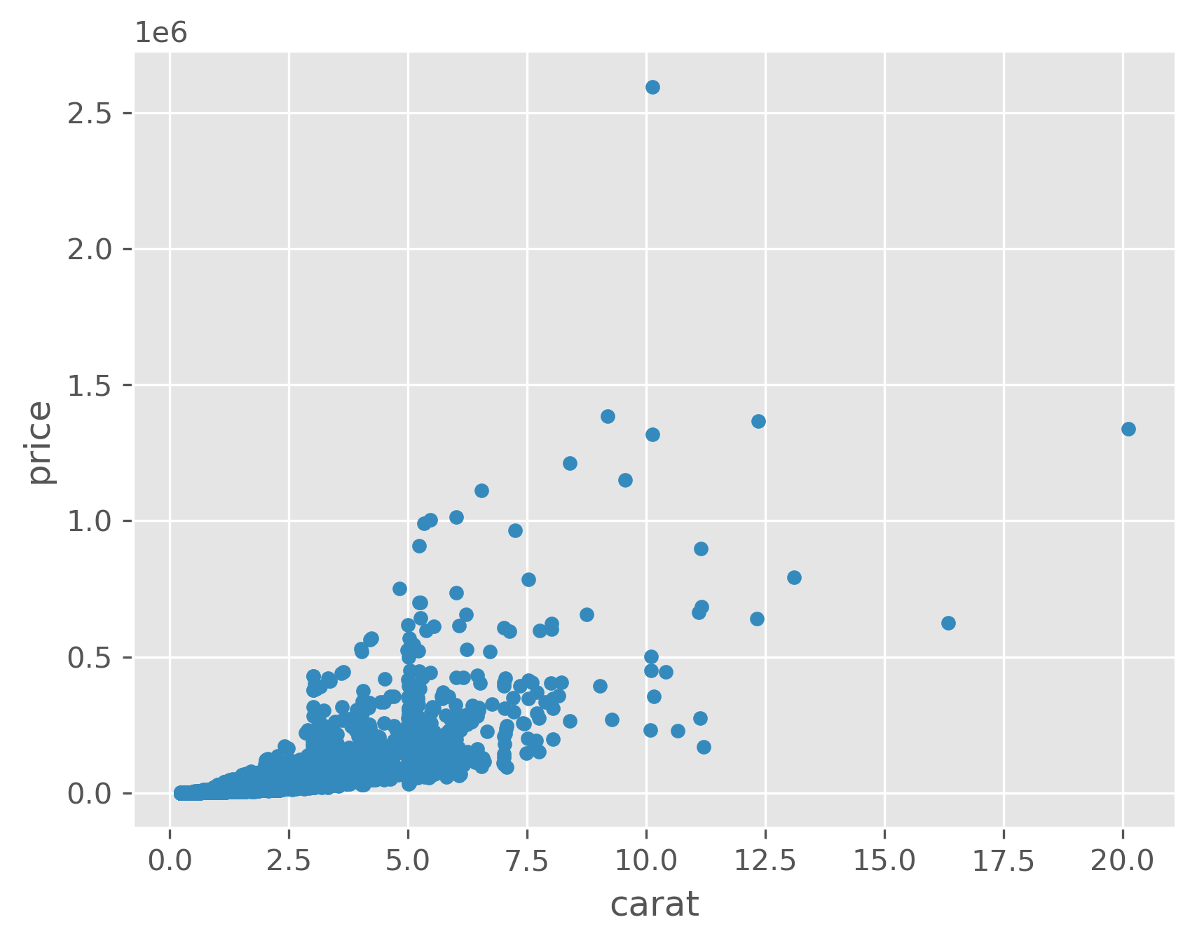
# scatter plot the relationship between carat and price
data.plot(kind='scatter', x='carat', y='price');
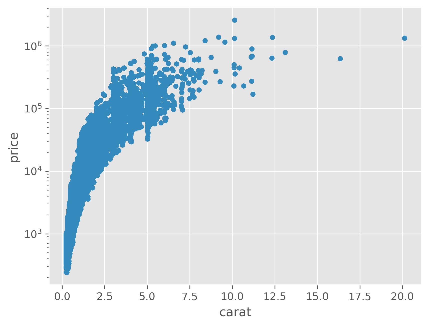
# do the same thing, but plot y on a log scale
data.plot(kind='scatter', x='carat', y='price', logy=True);
data.boxplot(column='log_price', by='color');
data.boxplot(column='log_price', by='cut');
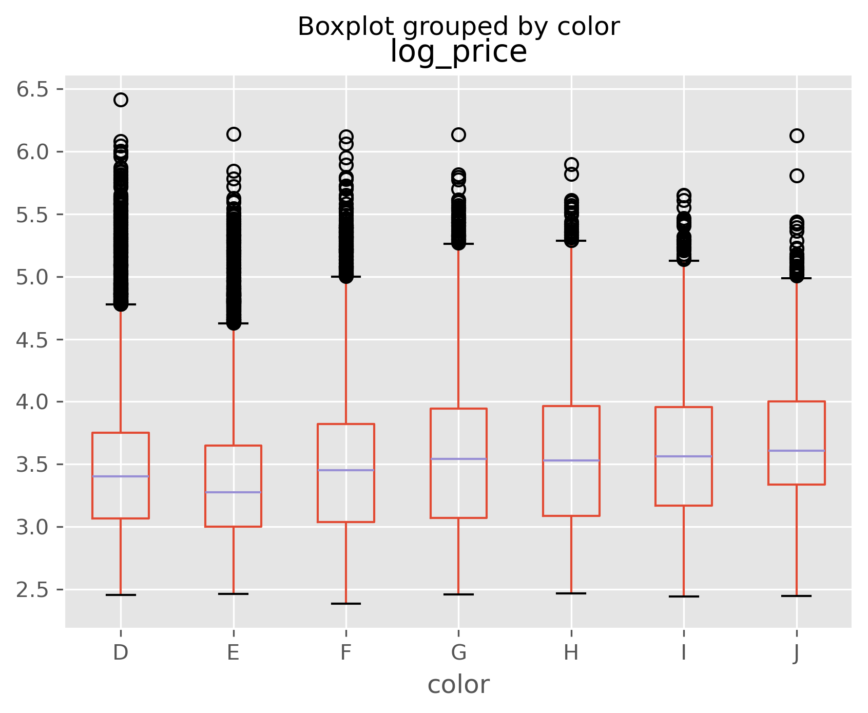
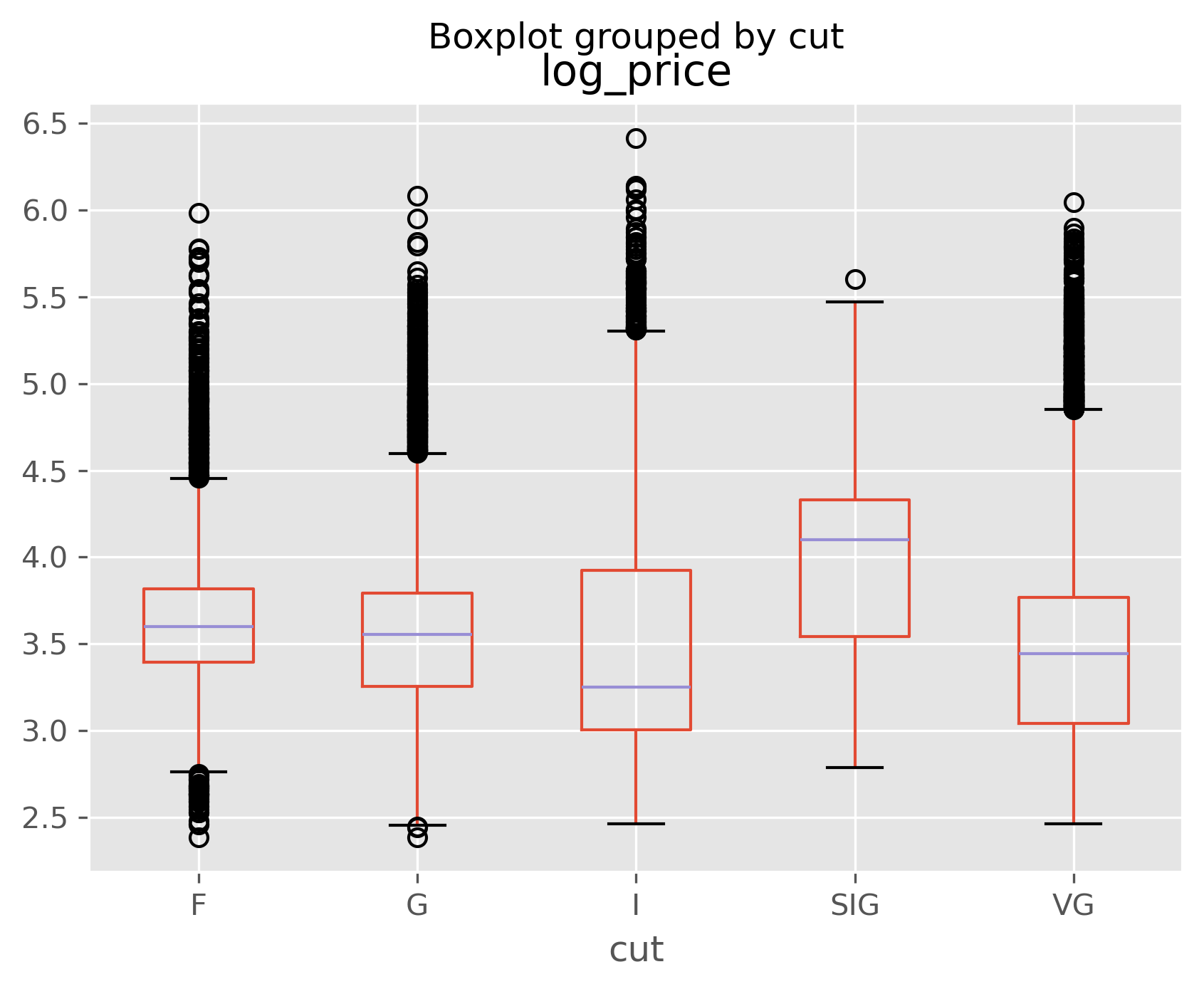
Challenge Question:
You can see from the above above that color and cut don’t seem to matter much to price. Can you think of a reason why this might be?
Solution#
Show code cell content
data.boxplot(column='carat', by='color');
plt.ylim(0, 3);
data.boxplot(column='carat', by='cut');
plt.ylim(0, 3);

from pandas.plotting import scatter_matrix

column_list = ['carat', 'price per carat', 'log_price']
scatter_matrix(data[column_list]);
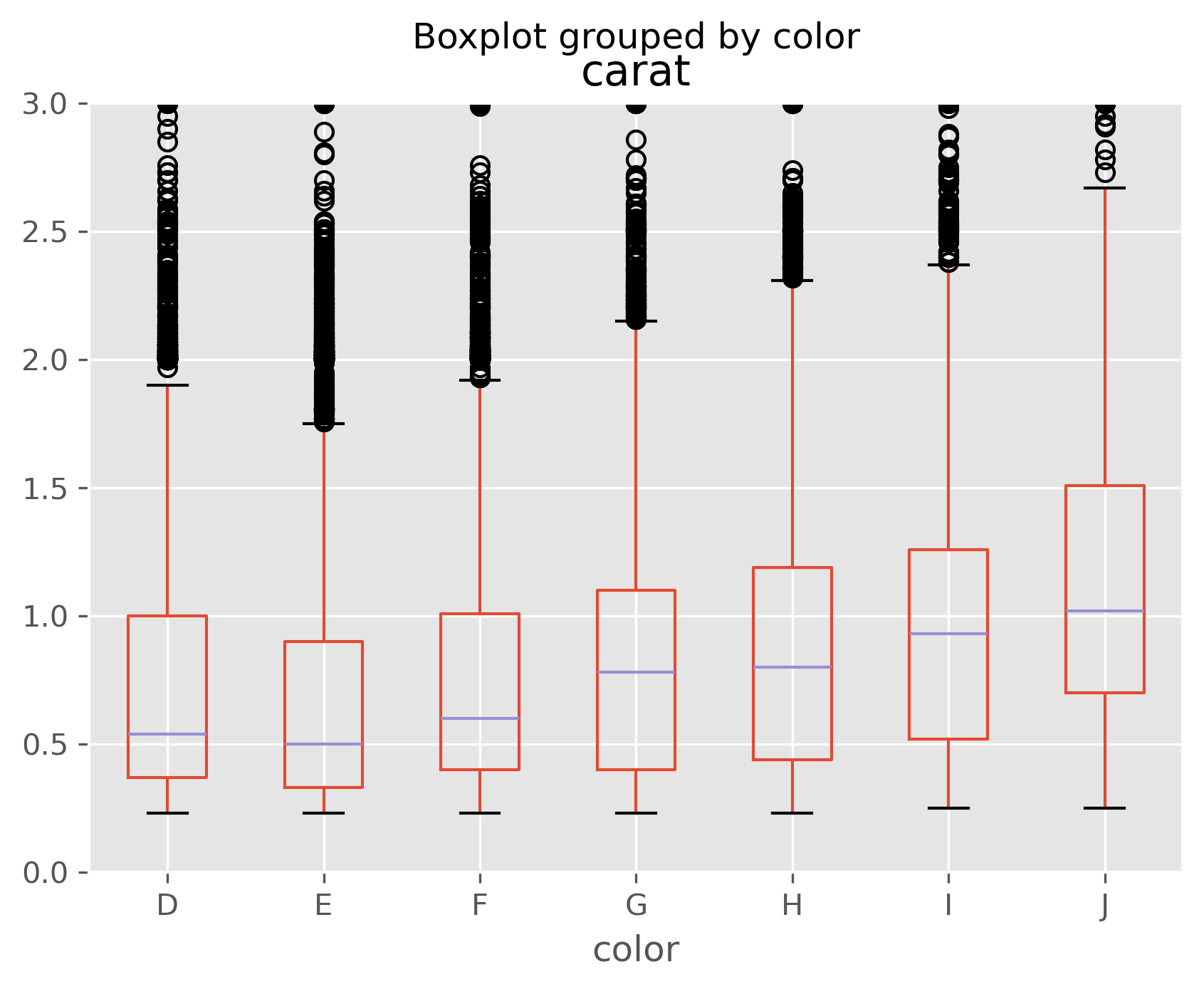
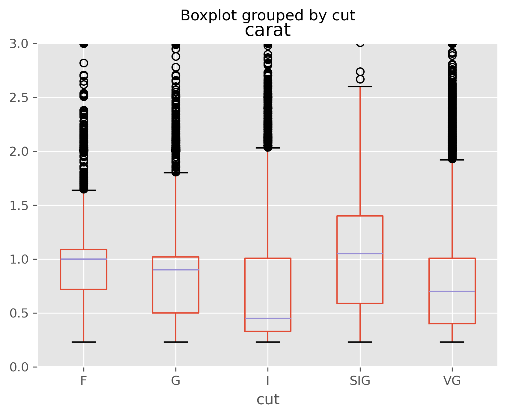
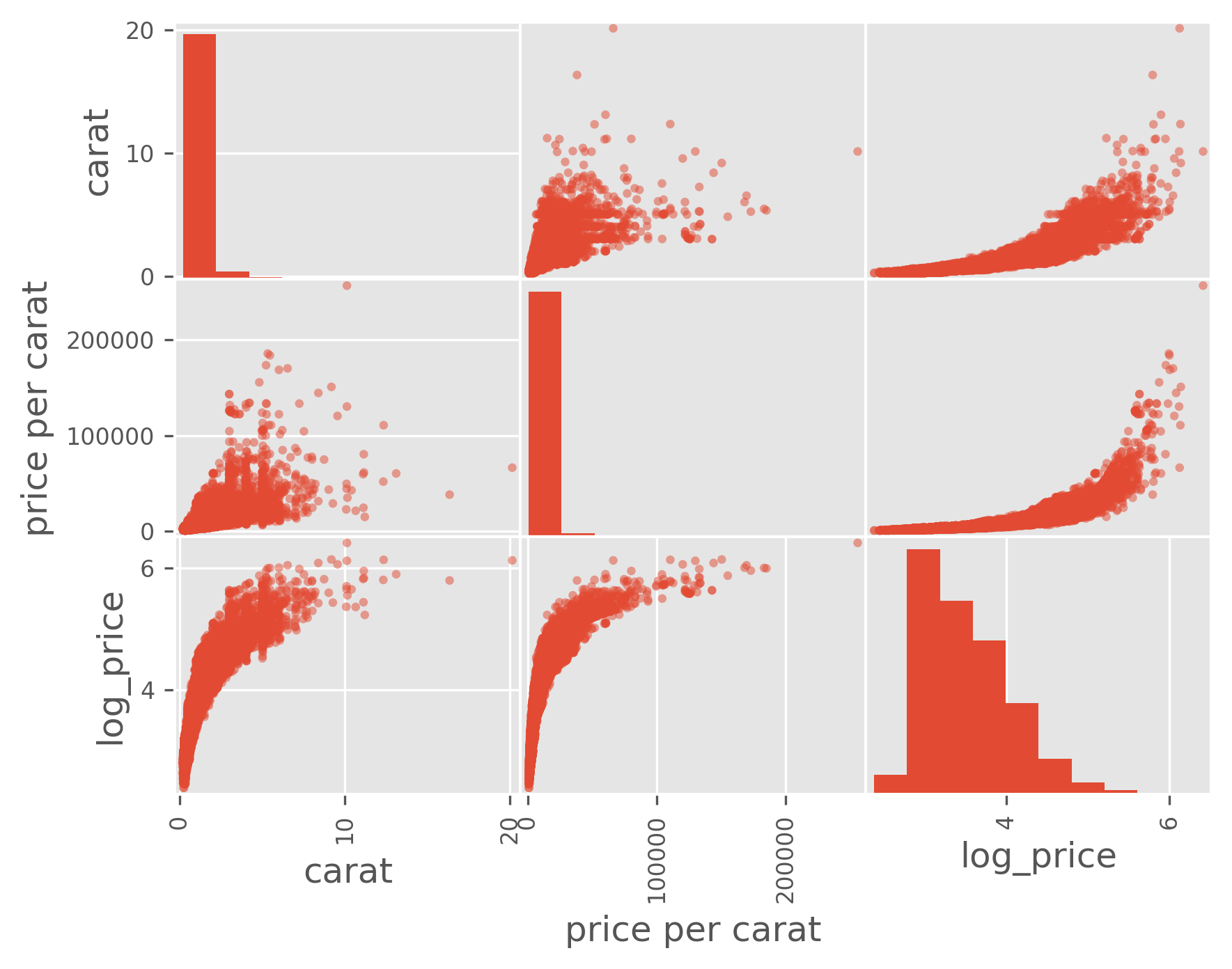
As we can see, especially in the last plot, size is strongly correlated with price, but size is inversely correlated with other quality measures. That is, if you’re going to stock a flawed or off-colored diamond, it is almost certainly a big one!
Final thoughts:#
There are lots and lots and lots of plotting libraries out there.
Matplotlib is the standard (and most full-featured), but it’s built to look and work like Matlab, which is not known for the prettiness of its plots.
There is an unofficial port of the excellent ggplot2 library from R to Python. It lacks some features, but does follow ggplot’s unique “grammar of graphics” approach.
Seaborn has become a pretty standard add-on to Matplotlib. ggplot-quality results, but with a more Python-y syntax. Focus on good-looking defaults relative to Matplotlib with less typing and swap-in stylesheets to give plots a consistent look and feel.
Bokeh has a focus on web output and large or streaming datasets.
plot.ly has a focus on data sharing and collaboration. May not be best for quick and dirty data exploration, but nice for showing to colleagues.
Warning
Very important: Plotting is lots of fun to play around with, but almost no plot is going to be of publication quality without some tweaking. Once you pick a package, you will want to spend time learning how to get labels, spacing, tick marks, etc. right. All of the packages above are very powerful, but inevitably, you will want to do something that seems simple and turns out to be hard.
Why not just take the plot that’s easy to make and pretty it up in Adobe Illustrator? Any plot that winds up in a paper will be revised many times in the course of revision and peer review. Learn to let the program do the hard work. You want code that will get you 90 - 95% of the way to publication quality.
Thankfully, it’s very, very easy to learn how to do this. Because plotting routines present such nice visual feedback, there are lots and lots of examples on line with code that will show you how to make gorgeous plots. Here again, documentation and StackOverflow are your friends!